Lower Putah Creek Watershed
Land Classification
Introduction
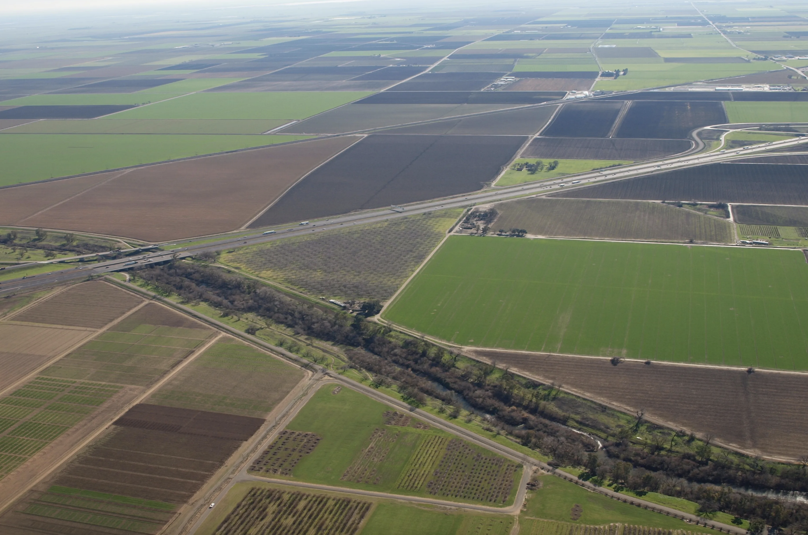
Putah Creek Watershed is located in west-central California, covering 638 square miles at a length of about 70 miles. Creek headwaters are nested in the Mayacamas Mountains, part of the Coast Range near 4,7000 ft. elevation, flowing east to the Berryessa Reservoir. Monticello Dam releases water from the lake to another dam, Putah Diversion Dam (PDD). The watershed is segmented into upper and lower watersheds, with lower Putah Creek residing below PDD consisting of 32 miles of creek ending in the Yolo Bypass, a tributary of the Sacramento River. Most of the annual flow in this subwatershed (~90%) can be attributed to the upper watershed hydrology.
Lower Putah Creek has a decades long history of legal conflict (Borchers, 2018) beginning with the Bureau of Reclamation Solano Project forming PDD and Berryessa Reservoir (1957). The project allocated water for agricultural, industrial, and municipal use and soon led to the drying of the creek (1989). The consequential impact on riparian wildlife catalyzed a local response from the non-profit Putah Creek Council (PCC) which moved to file a lawsuit against both Solano County Water Agency and Solano Irrigation District. PCC was joined in the lawsuit by the Regents of the University of California and many municipalities. In 1996, the case went to trial and the California Superior Court ordered a 50% increase in the PDD minimum release schedule. Thereafter the Putah Creek Accord (2000) established a flow regime more closely aligned with the creek’s historic flow regime and ensured seasonal pulse flows for anadromous fish.
Data Description
The HLSL30 v002 product provides 30-m Nadir Bidirectional Reflectance Distribution Function (BRDF)-Adjusted Reflectance (NBAR) and is derived from Landsat 8/9 Operational Land Imager (OLI) data products through the Harmonized Landsat Sentinel-2 (HLS) project. The sensor resolution is 30m, imagery resolution is 30m, and the temporal resolution is daily with an 8 day revisit time.
USGS Watershed Boundary Dataset (WBD) for 2-digit Hydrologic Unit - 18 is a dataset of hydrologic unit polygons and corresponding lines that define the boundary of each polygon. Polygon attributes include hydrologic unit codes (HUC), size (in the form of acres and square kilometers), name, downstream hydrologic unit code, type of watershed, non-contributing areas, and flow modifications.
Data Citation
NASA. (2024). HLSL30 v002 [Data set]. http://doi.org/10.5067/HLS/HLSL30.002
USGS. (2025). USGS Watershed Boundary Dataset (WBD) for 2-digit Hydrologic Unit - 18 (published 20250108) Shapefile [Data set]. https://prd-tnm.s3.amazonaws.com/StagedProducts/Hydrography/WBD/HU2/Shape/WBD_18_HU2_Shape.zip
Methods
The HU12 subwatershed within Hydrologic Unit Region 18 was loaded into a GeoDataFrame with geopandas. The watershed boundary dataset (WBD) was subset for Lower Putah Creek and geometries were dissolved into a single observation. earthaccess (a library for NASA’s Search API) retrieved data granules by dataset (HLSL30) and scoped the data to late 2023 (October to December) and the spatial bounds collected from the WBD GeoDataFrame.
Granule metadata was compiled cropped, scaled, masked, and merged into a spectral reflectance DataFrame of processed DataArrays. The DataFrame was grouped by band to concatenate across dates and produce a composite DataArray. Finally, with bands ranging across varying wavelengths, the Elbow Method was applied to select the optimal number of clusters. Data was clustered by spectral signature using the scikit-learn k-means algorithm.
Analysis
Imports
import os
import pickle
import re
import pathlib
import warnings

import earthaccess
from earthaccess import results
import earthpy as et
import geopandas as gpd
import cartopy.crs as ccrs
import geoviews as gv
import hvplot.pandas
import hvplot.xarray
import numpy as np
import pandas as pd
import rioxarray as rxr
import rioxarray.merge as rxrmerge
from tqdm.notebook import tqdm
import xarray as xr
from shapely.geometry import Polygon
from sklearn.cluster import KMeans
import matplotlib.pyplot as plt

warnings.simplefilter('ignore')
# Prevent Geospatial Data Abstraction Library (GDAL) from quitting due to momentary disruptions
os.environ["GDAL_HTTP_MAX_RETRY"] = "5"
os.environ["GDAL_HTTP_RETRY_DELAY"] = "1"
Include Cache Decorator
def cached(func_key, override=False):
    """
    A decorator to cache function results

    Parameters
    ==========
    key: str
      File basename used to save pickled results
    override: bool
      When True, re-compute even if the results are already stored
    """
    def compute_and_cache_decorator(compute_function):
        """
        Wrap the caching function

        Parameters
        ==========
        compute_function: function
          The function to run and cache results
        """
        def compute_and_cache(*args, **kwargs):
            """
            Perform a computation and cache, or load cached result.

            Parameters
            ==========
            args
              Positional arguments for the compute function
            kwargs
              Keyword arguments for the compute function
            """
            # Add an identifier from the particular function call
            if 'cache_key' in kwargs:
                key = '_'.join((func_key, kwargs['cache_key']))
            else:
                key = func_key

            path = os.path.join(
                et.io.HOME, et.io.DATA_NAME, 'jars', f'{key}.pickle')

            # Check if the cache exists already or override caching
            if not os.path.exists(path) or override:
                # Make jars directory if needed
                os.makedirs(os.path.dirname(path), exist_ok=True)

                # Run the compute function as the user did
                result = compute_function(*args, **kwargs)

                # Pickle the object
                with open(path, 'wb') as file:
                    pickle.dump(result, file)
            else:
                # Unpickle the object
                with open(path, 'rb') as file:
                    result = pickle.load(file)

            return result

        return compute_and_cache

    return compute_and_cache_decorator
Download Watershed Boundary
@cached('region_18', override=False)
def download_watershed_bounds(boundary_filename, huc):
    """
    Download a USGS watershed boundary dataset.

    Args:
    boundary_filename (str): USGS WBD shapefile name.
    huc (int): USGS Hydrologic Unit Code.

    Returns:
    geopandas.GeoDataFrame: Regional watershed boundary.
    """
    water_boundary_url = (
        "https://prd-tnm.s3.amazonaws.com/StagedProducts/Hydrography/WBD/"
        f"HU2/Shape/{boundary_filename}.zip"
    )

    # Download data
    wbd_dir = et.data.get_data(url=water_boundary_url)

    # Join shapefile path
    hu12_shape_path = os.path.join(wbd_dir, 'Shape', f'WBDHU{huc}.shp')

    # Load dataset

    # Pyogrio provides fast, bulk-oriented read and write access to GDAL
    # vector data sources, such as ESRI Shapefile
    hu12_gdf = gpd.read_file(hu12_shape_path, engine='pyogrio')

    return hu12_gdf
# Hydrologic Unit level "HU2" indicates a large region
region = '18'

boundary_filename = f'WBD_{region}_HU2_Shape'

# HU12: a very small subwatershed within a HU2 region
huc = 12

wbd_gdf = download_watershed_bounds(boundary_filename, huc)
# Select watershed

# Putah Creek-Lower Putah Creek
watershed = '180201620504'

sf_putah_gdf = (
    wbd_gdf[wbd_gdf[f'huc{huc}'] # select HU12 subregion
    .isin([watershed])] # subset for Lower Putah Creek
    .dissolve() # dissolve geometries into single observation
)
# Plot watershed

(
    sf_putah_gdf.to_crs(ccrs.Mercator())
    .hvplot(
        alpha=.2, fill_color='white', tiles='EsriImagery',
        crs=ccrs.Mercator())
    .opts(width=600, height=400)
)

Retrieve Multispectral Data
earthaccess.login(strategy="interactive", persist=True)

# Search for HLS tiles
sf_putah_gdf_results = earthaccess.search_data(
    short_name="HLSL30", # Harmonized Sentinal/Landsat multispectral dataset
    cloud_hosted=True,
    bounding_box=tuple(sf_putah_gdf.total_bounds),
    temporal=("2023-10-01", "2023-12-01"))
Compile Granule Metadata
@cached('granule_metadata', override=False)
def build_granule_metadata(hls_results):
    """
    Collect granule metadata from HLS tiles.

    Args:
    hls_results (List[DataGranule]): HLS search results list.

    Returns:
    granule_metadata (list): List of granule metadata dictionaries.
    """

    # Find all the metadata in the file
    granule_metadata = []

    # Loop through each granule
    for result in tqdm(hls_results):

        # Granule ID
        granule_id = result['umm']['GranuleUR']

        # Get datetime
        temporal_coverage = results.DataCollection.get_umm(
            result, 'TemporalExtent')
        granule_date = (pd.to_datetime(
            temporal_coverage['RangeDateTime']['BeginningDateTime']
        ).strftime('%Y-%m-%d'))

        print(f'Processing date {granule_date}. Granule ID: {granule_id}.')

        # Assemble granule polygon
        spatial_ext = results.DataCollection.get_umm(result, 'SpatialExtent')
        granule_geo = spatial_ext['HorizontalSpatialDomain']['Geometry']
        granule_points = granule_geo['GPolygons'][0]['Boundary']['Points']
        granule_coords = [tuple(point.values()) for point in granule_points]
        granule_polygon = Polygon(granule_coords)

        # Open granule files
        granule_files = earthaccess.open([result])

        # Use () to select the desired name and only output that name
        uri_re = re.compile(
            r"v2.0/(HLS.L30.*.tif)"
        )

        # Select unique tiles
        tile_id_re = re.compile(
            r"HLSL30.020/(HLS.L30..*.v2.0)/HLS"
        )

        # Grab band IDs
        band_id_re = re.compile(
            r"HLS.L30..*v2.0.(\D{1}.*).tif"
        )

        # Collect file metadata
        for uri in granule_files:

            # Make sure uri has full_name property first
            if (hasattr(uri, 'full_name')):
                file_name = uri_re.findall(uri.full_name)[0]
                tile_id = tile_id_re.findall(uri.full_name)[0]
                band_id = band_id_re.findall(uri.full_name)[0]

                # Only keep spectral bands and cloud Fmask
                # Exclude sun and view angles
                exclude_files = ['SAA', 'SZA', 'VAA', 'VZA']

                if band_id not in exclude_files:
                    granule_metadata.append({
                        'filename': file_name,
                        'tile_id': tile_id,
                        'band_id': band_id,
                        'granule_id': granule_id,
                        'granule_date': granule_date,
                        'granule_polygon': granule_polygon,
                        'uri': uri
                    })

    # Concatenate granule metadata
    granule_metadata_df = pd.DataFrame(
        data=granule_metadata, columns=[
            'filename', 'tile_id', 'band_id', 'granule_id',
            'granule_date', 'granule_polygon', 'uri'])

    granule_results_gdf = gpd.GeoDataFrame(
            granule_metadata_df,
            geometry=granule_metadata_df['granule_polygon'],
            crs="EPSG:4326")

    return granule_results_gdf
sf_putah_gdf_metadata = build_granule_metadata(sf_putah_gdf_results)
Open, Crop, and Mask Data
def process_image(uri, bounds_gdf, masked=True, scale=1):
    """
    Load, crop, and scale a raster image

    Parameters
    ----------
    uri: file-like or path-like
      File accessor
    bounds_gdf: gpd.GeoDataFrame
      Area of interest

    Returns
    -------
    cropped_da: rxr.DataArray
      Processed raster
    """
    # Load and scale
    da = rxr.open_rasterio(uri, masked=masked).squeeze() * scale

    # Obtain crs from raster
    raster_crs = da.rio.crs

    # Match coordinate reference systems
    bounds_gdf = bounds_gdf.to_crs(raster_crs)

    # Crop to site boundaries
    cropped_da = da.rio.clip_box(*bounds_gdf.total_bounds)

    return cropped_da
def process_mask(da, bits_to_mask):
    """
    Load a DataArray and process to a boolean mask

    Parameters
    ----------
    da: DataArray
      The input DataArray
    bits_to_mask: list of int
      The indices of the bits to mask if set

    Returns
    -------
    mask: np.array
      Boolean mask
    """
    # Get the mask as bits
    bits = (
        np.unpackbits(
            (
                # Get the mask as an array
                da.values
                # of 8-bit integers
                .astype('uint8')
                # with an extra axis to unpack the bits into
                .reshape(da.shape + (-1,))
            ),
            # List the least significant bit first to match the user guide
            bitorder='little',
            # Expand the array in a new dimension
            axis=-1)
    )

    # Calculate the product of the mask and bits to mask
    mask = np.prod(
        # Multiply bits and check if flagged
        bits[..., bits_to_mask]==0,
        # From the last to the first axis
        axis=-1
    )

    return mask
# Harmonized Landsat Sentinel-2 (HLS) band code name L8
bands = {
    'B01': 'aerosol',
    'B02': 'red',
    'B03': 'green',
    'B04': 'blue',
    # Near-infrared narrow (0.85 – 0.88 micrometers)
    'B05': 'nir',
    # Short-wave infrared (SWIR) wavelength 1.57 – 1.65 µm
    'B06': 'swir1',
    # SWIR (2.11 – 2.29 µm)
    'B07': 'swir2',
    'B09': 'cirrus',
    # Thermal infrared 1 (10.60 – 11.19 µm)
    'B10': 'thermalir1',
    # Thermal infrared 2 (11.50 – 12.51 µm)
    'B11': 'thermalir2'
}

# HLS Quality Assessment layer bits
bits_to_mask = [
    1, # Cloud
    2, # Adjacent to cloud/shadow
    3  # Cloud shadow
]
@cached('sf_putah_reflectance_da_df', override=False)
def compute_reflectance_da(file_df, boundary_gdf):
    """
    Connect to files over VSI (Virtual Filesystem Interface),
    crop, cloud mask, and wrangle data.

    Returns a reflectance DataArray within file DataFrame.

    Parameters
    ==========
    file_df : pd.DataFrame
        File connection and metadata
    boundary_gdf : gpd.GeoDataFrame
        Boundary use to crop the data
    """
    granule_da_rows= []

    # unique dated data granules
    tile_groups = file_df.groupby(['granule_date', 'tile_id'])

    for (granule_date, tile_id), tile_df in tqdm(tile_groups):
        print(f'Processing granule {tile_id} {granule_date}')

        # Grab Fmask row from tile group
        Fmask_row = tile_df.loc[tile_df['band_id'] == 'Fmask']
        # Load cloud path
        cloud_path = Fmask_row.uri.values[0]
        cloud_da = process_image(cloud_path, boundary_gdf, masked=False)
        # Compute cloud mask
        cloud_mask = process_mask(cloud_da, bits_to_mask)

        # Load spectral bands
        band_groups = tile_df.groupby('band_id')

        for band_name, band_df in band_groups:
            for index, row in band_df.iterrows():
                # Process band and retain band scale
                cropped_da = process_image(row.uri, boundary_gdf, scale=0.0001)
                cropped_da.name = band_name

                # Apply mask on band to remove unwanted cloud data
                row['da'] = cropped_da.where(~cropped_da.isin(cloud_mask))

                # Store the resulting DataArray
                granule_da_rows.append(row.to_frame().T)

    # Reassemble the metadata DataFrame
    return pd.concat(granule_da_rows)
sf_putah_reflectance_da_df = compute_reflectance_da(sf_putah_gdf_metadata, sf_putah_gdf)
Create Composite Data
@cached('sf_putah_reflectance_da', override=False)
def create_composite_da(granule_da_df):
    """
    Create a composite DataArray from a DataFrame containing granule
    metadata and corresponding DataArrays.

    Args:
    granule_da_df (pandas.DataFrame): Granule metadata DataFrame.

    Returns:
    xarray.DataArray: Composite granule DataArray.
    """
    composite_das = []

    for band, band_df in tqdm(granule_da_df.groupby('band_id')):
        merged_das = []

        if (band != 'Fmask'):
            for granule_date, date_df in tqdm(band_df.groupby('granule_date')):

                # For each date merge granule DataArrays
                merged_da = rxrmerge.merge_arrays(list(date_df.da))

                # Mask all negative values
                merged_da = merged_da.where(merged_da > 0)
                merged_das.append(merged_da)

            # Create composite images across dates (by median date)
            # to fill cloud gaps
            composite_da = xr.concat(
                merged_das, dim='granule_date').median('granule_date')

            # Add the band as a dimension
            composite_da['band'] = int(band[1:])

            # Name the composite DataArray
            composite_da.name = 'reflectance'

            composite_das.append(composite_da)

    # Concatenate on the band dimension
    return xr.concat(composite_das, dim='band')
sf_putah_reflectance_da = create_composite_da(sf_putah_reflectance_da_df)

# Drop thermal bands
sf_putah_reflectance_da = sf_putah_reflectance_da.drop_sel(band=[10, 11])
Cluster Data with k-means
# Convert spectral DataArray to a tidy DataFrame
sf_putah_reflectance_df = (
    sf_putah_reflectance_da.to_dataframe()
    .reflectance # select reflectance values
    .unstack('band')
).dropna()

sf_putah_reflectance_df
| band | 1 | 2 | 3 | 4 | 5 | 6 | 7 | 9 | |
|---|---|---|---|---|---|---|---|---|---|
| y | x | ||||||||
| 4267125.0 | 589365.0 | 0.02125 | 0.03555 | 0.07470 | 0.07630 | 0.29535 | 0.18025 | 0.09880 | 0.00135 |
| 589395.0 | 0.02010 | 0.03525 | 0.07950 | 0.07975 | 0.29670 | 0.17295 | 0.09595 | 0.00150 | |
| 589425.0 | 0.01885 | 0.03175 | 0.08225 | 0.07940 | 0.30055 | 0.16765 | 0.09475 | 0.00160 | |
| 589455.0 | 0.01925 | 0.03115 | 0.08100 | 0.07760 | 0.30390 | 0.16615 | 0.09505 | 0.00145 | |
| 589485.0 | 0.01835 | 0.03405 | 0.07600 | 0.07630 | 0.30405 | 0.16055 | 0.09225 | 0.00145 | |
| ... | ... | ... | ... | ... | ... | ... | ... | ... | ... |
| 4263015.0 | 622875.0 | 0.04760 | 0.05740 | 0.07550 | 0.09130 | 0.12760 | 0.19750 | 0.16850 | 0.00170 |
| 622905.0 | 0.04510 | 0.05390 | 0.07095 | 0.08560 | 0.12115 | 0.18850 | 0.15985 | 0.00160 | |
| 622935.0 | 0.04305 | 0.05155 | 0.06880 | 0.08360 | 0.11820 | 0.18400 | 0.15485 | 0.00150 | |
| 622965.0 | 0.04380 | 0.05205 | 0.06930 | 0.08570 | 0.11185 | 0.18675 | 0.15790 | 0.00165 | |
| 622995.0 | 0.04460 | 0.05350 | 0.07650 | 0.08970 | 0.15845 | 0.19795 | 0.15795 | 0.00185 |
154836 rows × 8 columns
# Collect the total squared clustering error for each k
k_inertia = []

# Experiment with different k values
k_values = list(range(2, 9))

for k in k_values:

    # Create model with k clusters
    k_means = KMeans(n_clusters = k)

    model_vars = (
        sf_putah_reflectance_df
        [[1, 2, 3, 4, 5, 6, 7, 9]])

    # Fit model
    k_means.fit(model_vars)

    # Calculate inertia
    k_inertia.append(k_means.inertia_)

plt.scatter(x=k_values, y=k_inertia)
plt.title('Cluster Inertia')
plt.xlabel("Clusters")
plt.ylabel("Total Squared Error")
plt.show()
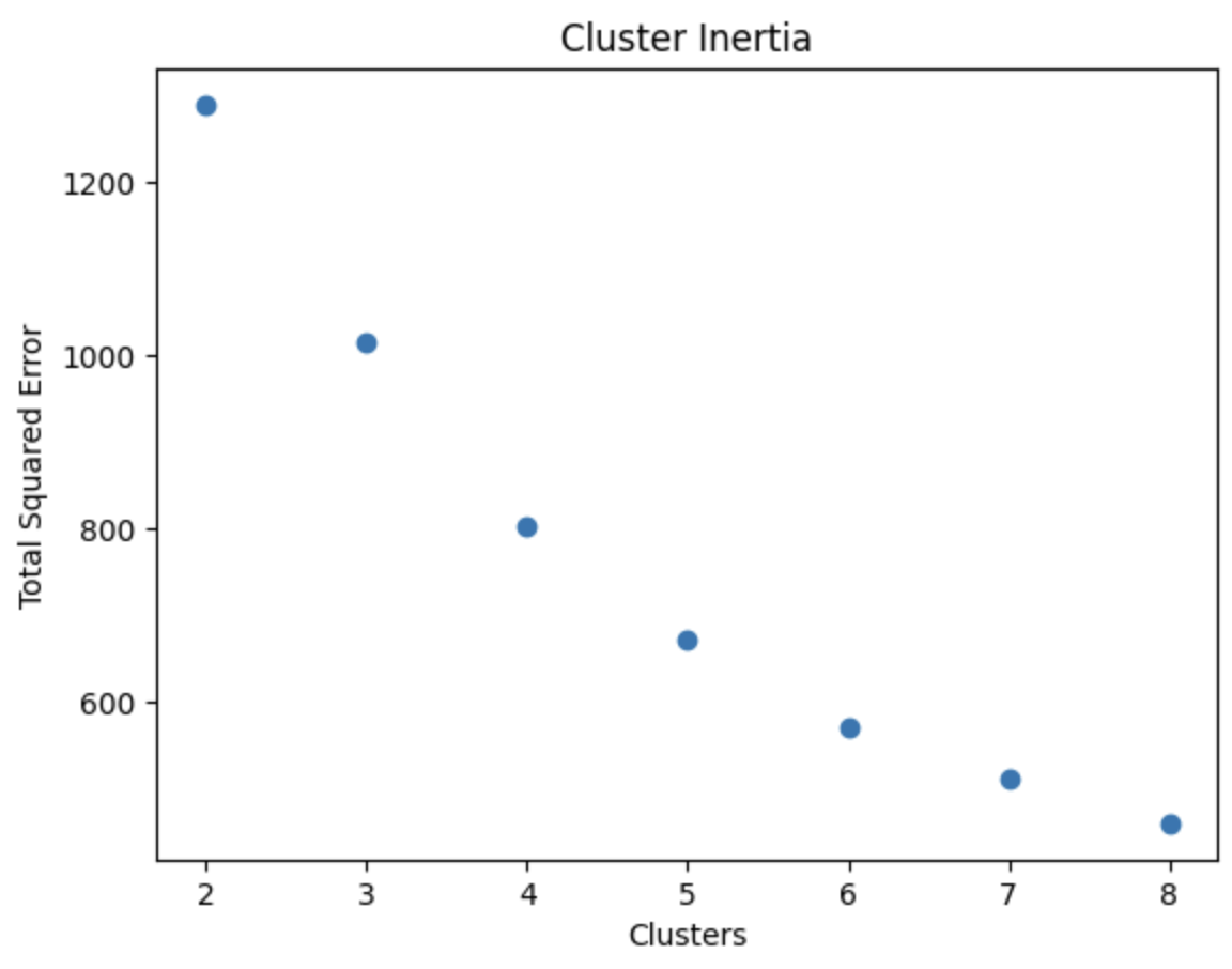
# k-means model with k clusters
k_means = KMeans(n_clusters = 5)

model_vars = (
    sf_putah_reflectance_df
    [[1, 2, 3, 4, 5, 6, 7, 9]])

# Fit the model to the spectral bands
k_means.fit(model_vars)

# Add the cluster labels to the dataframe
sf_putah_reflectance_df['cluster'] = k_means.labels_

# Inspect labels
sf_putah_reflectance_df
| band | 1 | 2 | 3 | 4 | 5 | 6 | 7 | 9 | cluster | |
|---|---|---|---|---|---|---|---|---|---|---|
| y | x | |||||||||
| 4267125.0 | 589365.0 | 0.02125 | 0.03555 | 0.07470 | 0.07630 | 0.29535 | 0.18025 | 0.09880 | 0.00135 | 0 |
| 589395.0 | 0.02010 | 0.03525 | 0.07950 | 0.07975 | 0.29670 | 0.17295 | 0.09595 | 0.00150 | 0 | |
| 589425.0 | 0.01885 | 0.03175 | 0.08225 | 0.07940 | 0.30055 | 0.16765 | 0.09475 | 0.00160 | 0 | |
| 589455.0 | 0.01925 | 0.03115 | 0.08100 | 0.07760 | 0.30390 | 0.16615 | 0.09505 | 0.00145 | 0 | |
| 589485.0 | 0.01835 | 0.03405 | 0.07600 | 0.07630 | 0.30405 | 0.16055 | 0.09225 | 0.00145 | 0 | |
| ... | ... | ... | ... | ... | ... | ... | ... | ... | ... | ... |
| 4263015.0 | 622875.0 | 0.04760 | 0.05740 | 0.07550 | 0.09130 | 0.12760 | 0.19750 | 0.16850 | 0.00170 | 4 |
| 622905.0 | 0.04510 | 0.05390 | 0.07095 | 0.08560 | 0.12115 | 0.18850 | 0.15985 | 0.00160 | 3 | |
| 622935.0 | 0.04305 | 0.05155 | 0.06880 | 0.08360 | 0.11820 | 0.18400 | 0.15485 | 0.00150 | 3 | |
| 622965.0 | 0.04380 | 0.05205 | 0.06930 | 0.08570 | 0.11185 | 0.18675 | 0.15790 | 0.00165 | 3 | |
| 622995.0 | 0.04460 | 0.05350 | 0.07650 | 0.08970 | 0.15845 | 0.19795 | 0.15795 | 0.00185 | 0 |
154836 rows × 9 columns
Plot Spectral Clusters
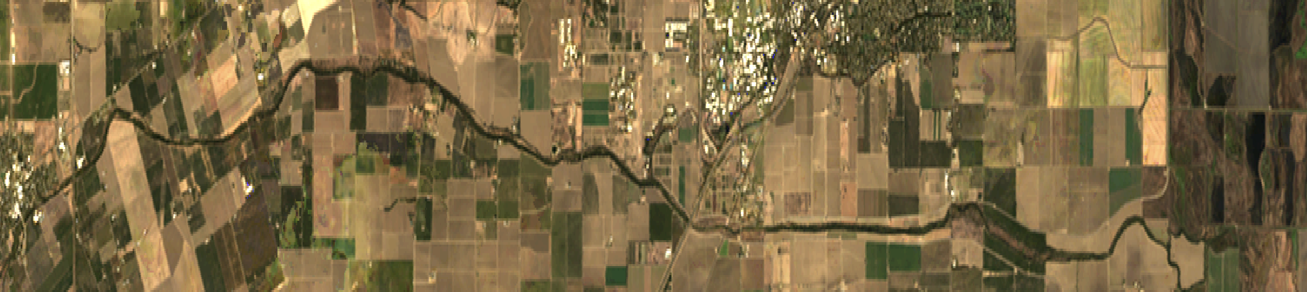
rgb = sf_putah_reflectance_da.sel(band=[4, 3, 2]) # blue, green, red
rgb_uint8 = (rgb * 255).astype(np.uint8).where(rgb!=np.nan)
# Brighten RGB image
rgb_bright = rgb_uint8 * 5
rgb_sat = rgb_bright.where(rgb_bright < 255, 255)
rgb_sat.hvplot.rgb(
x='x', y='y', bands='band',
data_aspect=1,
max_height=500,
max_width=10000,
xaxis=None, yaxis=None)
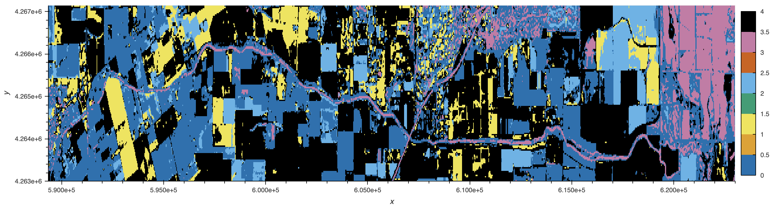
sf_putah_reflectance_df.cluster.to_xarray().sortby(['x', 'y']).hvplot(
cmap="Colorblind", aspect='equal', max_height=500, max_width=10000)
Discussion
The spectral signatures plot depicts observed clusters in the lower Putah Creek watershed. With bands ranging across varying wavelengths, cluster inertia was calculated to determine the optimal number of clusters. Five clusters were selected to best represent the scope of the spectral bands (aerosol, red, green, blue, and infrared) reflected in the landscape. The watershed is mostly flat and surrounded by agriculture, with the exception of the Yolo Bypass Wildlife Area (see plot on right). The area is composed of an assortment of habitats such as seasonal and permanent wetlands, vernal pools, and riparian forest. This variation is not easily discernable in the clustering however, likely due to managed seasonal flooding for migratory waterfowl.
Yolo Bypass Wildlife Area is managed by the California Department of Fish and Wildlife as part of a larger endeavor to steward habitats in the Yolo Basin, located in the northern area of the Sacramento-San Joaquin River Delta. Yolo Bypass maintains 60,000 acres for the Sacramento River during high flood events and drains back into the river and the Delta. Beyond flood management, the bypass supplies key ecological benefits to fish, and the lower Putah Creek plays a role in this service. During the recent rehabilitation of the creek, native fishes recovered and reversed a dominance of nonnative species in the creek and their growing presence in the bypass. Yolo Bypass provides nursery area for young fish in the north of the Delta as well as good habitat for salmon migrating to the bay. Recognizing the multi-purpose benefits delivered by the bypass in addition to the pressing mandate to build resiliency under climate change, Congress authorized a comprehensive study of the Yolo Bypass (2020) to be conducted by the US Army Corps of Engineers (2023-2029). The study will engage federal, state, and local stakeholders to create recommendations for bypass project purposes and address multiple public needs in the future of the state’s primary floodplain.
References
Barrett, A., Battisto, C., J. Bourbeau, J., Fisher, M., Kaufman, D., Kennedy, J., … Steiker, A. (2024). earthaccess (Version 0.12.0) [Computer software]. Zenodo. https://doi.org/10.5281/zenodo.8365009
Borchers, J. (2018, November 25). Case Study: Solano County Water Agency. Sierra Institute. https://sierrainstitute.us/new/wp-content/uploads/2021/10/Solano-County-Water-Agency-Summary-Report-11-25-18-NO-RESPONDENT-FOOTNOTES.pdf
da Costa-Luis, C., Larroque, S., Altendorf, K., Mary, H., Sheridan, R., Korobov, M., … McCracken, J. (2024). tqdm: A fast, Extensible Progress Bar for Python and CLI (Version 4.67.1) [Computer software]. Zenodo. https://zenodo.org/records/14231923
Delta Stewardship Council. (2025, January 28). Yolo Bypass inundation. https://viewperformance.deltacouncil.ca.gov/pm/yolo-bypass-inundation
Gillies, S., van der Wel, C., Van den Bossche, J., Taves, M. W., Arnott, J., & Ward, B. C. (2025). Shapely (Version 2.0.7) [Computer software]. Zenodo. https://doi.org/10.5281/zenodo.14776272
Harris, C. R., Millman, K. J., J. van der Walt, S., Gommers, R., Virtanen, P., Cournapeau, D., … Oliphant, T. E. (2020). Array programming with NumPy. Nature, 585, 357–362. https://doi.org/10.1038/s41586-020-2649-2
Hoyer, S. & Hamman, J., (2017). xarray: N-D labeled arrays and datasets in Python. Journal of Open Research Software. 5(1), 10. https://doi.org/10.5334/jors.148
Hunter, J. D. (2024). Matplotlib: A 2D graphics environment (Version 3.9.2) [Computer software]. Zenodo. https://zenodo.org/records/13308876
Jordahl, K., Van den Bossche, J., Fleischmann, M., Wasserman, J., McBride, J., Gerard, J., … Leblanc, F. (2024). geopandas/geopandas: v1.0.1 (Version 1.0.1) [Computer software]. Zenodo. https://doi.org/10.5281/zenodo.12625316
Met Office. (2024). Cartopy: a cartographic python library with a Matplotlib interface (Version 0.24.1) [Computer software]. Zenodo. https://doi.org/10.5281/zenodo.13905945
Pottinger, L. (2019, July 29). The Yolo Bypass: It’s a floodplain! It’s farmland! It’s an ecosystem! Public Policy Institute of California. https://www.ppic.org/blog/the-yolo-bypass-its-a-floodplain-its-farmland-its-an-ecosystem
Putah Creek Council. (n.d.). The Putah Creek Watershed. https://putahcreekcouncil.org/who-we-are/putah-creek-watershed
Python Software Foundation. (2024). Python (Version 3.12.8) [Computer software]. https://docs.python.org/release/3.12.6
Rudiger, P., Hansen, S. H., Bednar, J. A., Steven, J., Liquet, M., Little, B., … Bampton, J. (2024). holoviz/geoviews: Version 1.13.0 (Version 1.13.0) [Computer software]. Zenodo. https://doi.org/10.5281/zenodo.13782761
Rudiger, P., Liquet, M., Signell, J., Hansen, S. H., Bednar, J. A., Madsen, M. S., … Hilton, T. W. (2024). holoviz/hvplot: Version 0.11.0 (Version 0.11.0) [Computer software]. Zenodo. https://doi.org/10.5281/zenodo.13851295
Rypel, A. (2023, July 8). Putah Creek’s rebirth: A model for reconciling other degraded streams? UC Davis Center for Watershed Sciences. https://californiawaterblog.com/2023/07/08/putah-creeks-rebirth-a-model-for-reconciling-other-degraded-streams
Sacramento River Watershed Program. (n.d.). Putah Creek Watershed. https://sacriver.org/explore-watersheds/westside-subregion/putah-creek-watershed
Snow, A. D., Scott, R., Raspaud, M., Brochart, D., Kouzoubov, K., Henderson, S., … Weidenholzer, L. (2024). corteva/rioxarray: 0.18.1 Release (Version 0.18.1) [Computer software]. Zenodo. https://doi.org/10.5281/zenodo.4570456
The pandas development team. (2024). pandas-dev/pandas: Pandas (Version 2.2.2) [Computer software]. Zenodo. https://doi.org/10.5281/zenodo.3509134
The scikit-learn developers. (2024). scikit-learn (1.5.2). [Computer software]. Zenodo. https://doi.org/10.5281/zenodo.13749328
US Army Corps of Engineers. (n.d.). Yolo Bypass comprehensive study. https://www.spk.usace.army.mil/Missions/Civil-Works/Yolo-Bypass
Wasser, L., Max, J., McGlinchy, J., Palomino, J., Holdgraf, C., & Head, T. (2021). earthlab/earthpy: Soft release of earthpy (Version 0.9.4) [Computer software]. Zenodo. https://zenodo.org/records/5544946
Yolo Basin Foundation. (n.d.). About the Yolo Bypass Wildlife Area. https://yolobasin.org/yolobypasswildlifearea