Blue Oak
Habitat Suitability
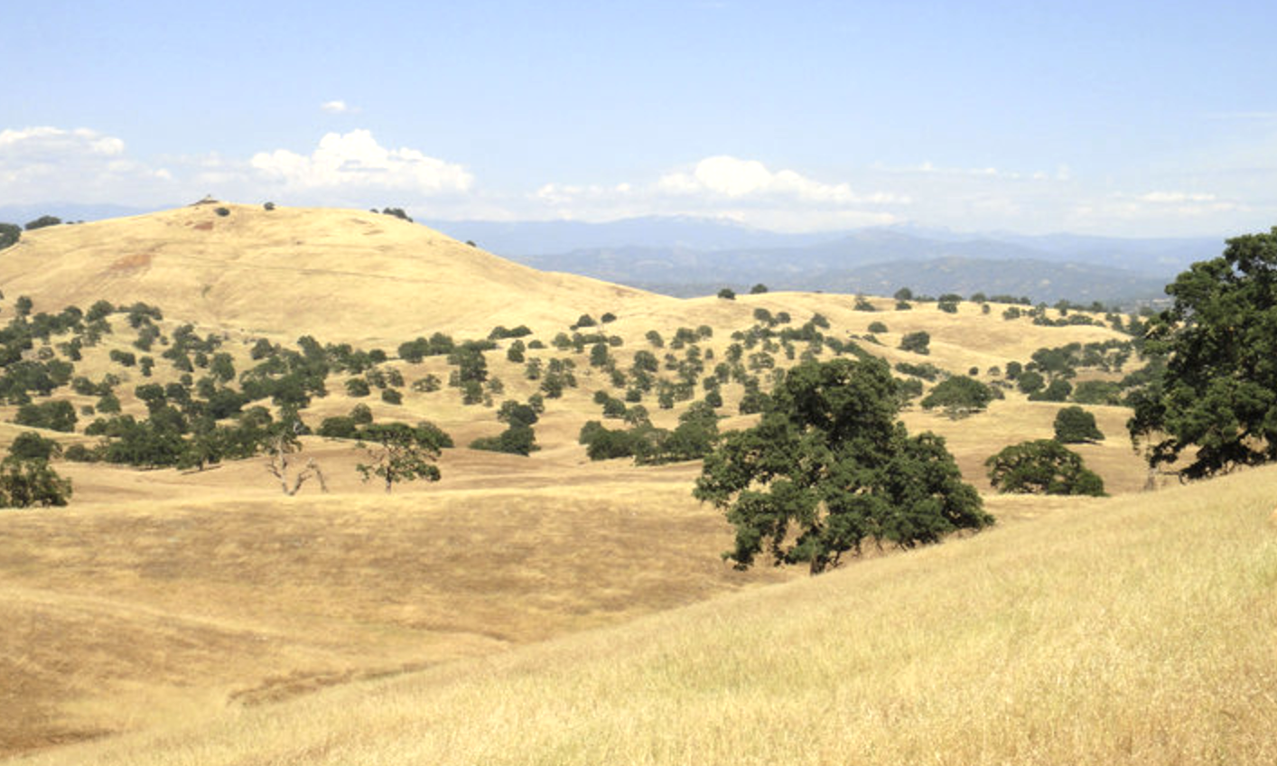
The blue oak (Quercus douglasii) is a deciduous drought-tolerant tree endemic to California. Blue oaks can be identified by their blue-green foliage, slightly to deeply lobed leaves, textured and pale gray bark, typical height between 20-60 ft., and natural settings of dry, rocky, and somewhat acidic to neutral soils. Acorns germinate in fall, appear in winter, and are propagated by species like the California Scrub-Jay which can plant up to 3,300 oaks each year (Tallamy, 2021). Most seasonal development occurs during March through May when water uptake is high and air temperatures rise.
Across North America, oaks support more life than any other tree due to their caterpillar abundance. Caterpillars are necessary to sustain terrestrial food webs: they are a key survival food for baby birds and also support larger animals like bears. Within California, oak woodlands have one of the highest levels of biodiversity in the state, sustaining over 5,000 plant and animal species. The blue oak alone is estimated to host approximately 170 moth and butterfly species. This species can be found among plant communities such as chaparral, foothill woodland, and oak woodland at elevations of 500-2000 ft. in the north and up to 5000 ft. in the south. The blue oak is dispersed throughout the state including in the central Sierra Nevada Eldorado National Forest and the central Coast and Transverse Ranges in Los Padres National Forest.
Data Description
National Forest System Land Units includes proclaimed national forest, purchase unit, national grassland, land utilization project, research and experimental area, national preserve, and other land area. An NFS Land Unit is nationally significant classification of Federally owned forest, range, and related lands that are administered by the USDA Forest Service or designated for administration through the Forest Service.
MACAV2-METDATA DAILY/MONTHLY is a downscaled climate dataset that covers CONUS at 4 kilometers (1/24 degree) resolution. Temporal coverage encompasses historical model output (1950-2005) and projections (2006-2099) for climate normals represented as monthly averages of daily values.
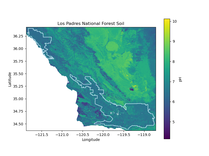
Probabilistic Remapping of SSURGO (POLARIS) soil properties is a dataset of 30‐m probabilistic soil property maps over the contiguous United States (CONUS). The mapped variables over CONUS include soil texture, organic matter, pH, saturated hydraulic conductivity, Brooks‐Corey and Van Genuchten water retention curve parameters, bulk density, and saturated water content.
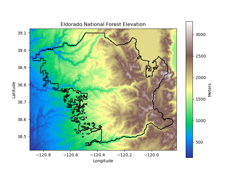
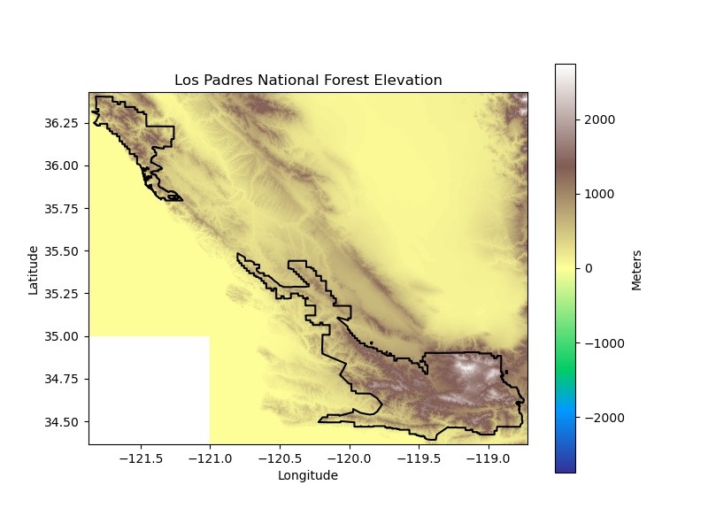
The SRTM 1 Arc-Second Global product offers global coverage of void filled elevation data at a resolution of 1 arc-second (30 meters). The Shuttle Radar Topography Mission (SRTM) was flown aboard the space shuttle Endeavour February 11-22, 2000.
Data Citation
Abatzoglou, J. T. (2017). REACCH Climatic Modeling CMIP5 MACAV2-METDATA DAILY/MONTHLY Catalog [Data set]. https://www.reacchpna.org/thredds/reacch_climate_CMIP5_macav2_catalog2.html
Chaney, N. W., Minasny, B., Herman, J. D., Nauman, T. W., Brungard, C. W., Morgan, C. L. S., McBratney, A. B., Wood, E. F., & Yimam, Y. (2019, February 5). POLARIS soil properties: 30-m probabilistic maps of soil properties over the contiguous United States. Water Resources Research, 55(4). https://doi.org/10.1029/2018WR022797
NASA. (2024). SRTM 1 Arc-Second Global [Data set]. https://doi.org/10.5066/F7PR7TFT
USDA Forest Service. (2024). National Forest System Land Units [Data set]. https://data.fs.usda.gov/geodata/edw/edw_resources/shp/S_USA.NFSLandUnit.zip
Methods
Downscaled climate models were compared by site under the RCP 4.5 emissions scenario for two periods (2036-2066 and 2066-2096), examining winter and summer mean temperatures (and change relative to historical by °F) as well as winter precipitation (and percent change relative to the historical value). The land units shapefile was extracted and read into a GeoDataFrame with geopandas and subset for site locations. earthaccess (a library for NASA’s Search API) retrieved digital elevation models by dataset (SRTMGL1) which were scoped to spatial bounds collected from the unit sites. Mean soil data was selected for pH, depth, and location through POLARIS.
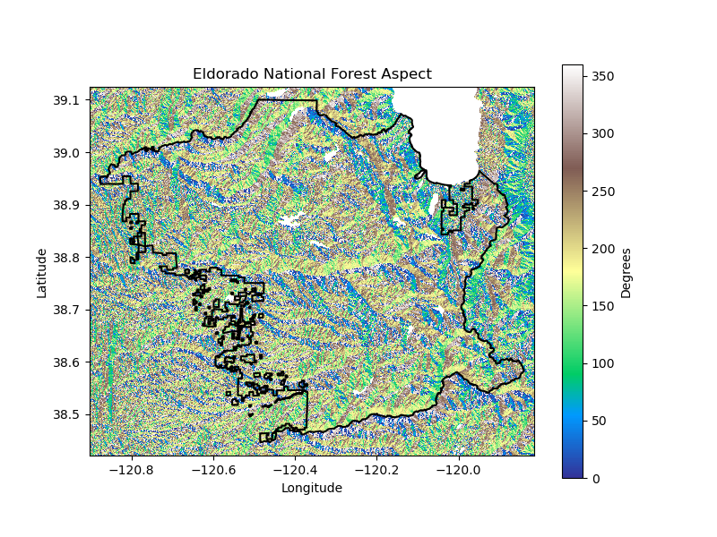
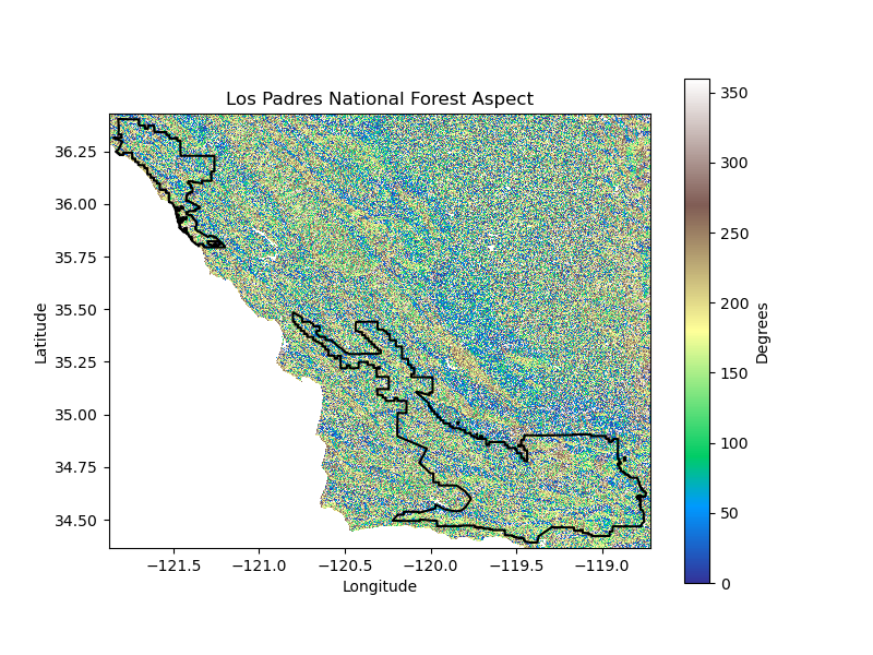
Data granules were processed into soil and elevation rasters through masking, scaling, cropping, and merging. The xarray-spatial aspect function calculated aspect in degrees for each cell in a site elevation raster. Projected climate scenarios (medium and high emissions) for a monthly average of daily maximum near-surface air temperature in 2096-2099 were obtained from MACAV2, scoped to site boundaries, assigned a longitude coordinate range aligned with existing rasters, and converted from Kelvin to Fahrenheit. Sites and corresponding attributes were subsequently plotted using the hvplot API and exported to rasters.
Given optimal characteristics for each site variable, a habitat suitability score was identified for each site leveraging a fuzzy Gaussian function to assign scores for each raster cell based on proximity to ideal site values. For each site and medium emissions scenario, variable rasters were harmonized across resolution and projection, suitability layers calculated and multiplied, and then combined into a final raster.
Analysis
Imports
import warnings
warnings.simplefilter(action='ignore', category=FutureWarning)

import os
import pathlib
import zipfile
from glob import glob
import tqdm as notebook_tqdm

import pandas as pd
import numpy as np
import geopandas as gpd
import rioxarray as rxr
from rioxarray.merge import merge_arrays
import xarray as xr
import xrspatial

import matplotlib.pyplot as plt
import hvplot.pandas
import hvplot.xarray
import cartopy.crs as ccrs
import geoviews as gv

import earthaccess
Set Paths
# Plots
plots_dir = os.path.join(
    # Home directory
    pathlib.Path.home(),
    'Projects',
    # Project directory
    'habitat-suitability',
    'plots'
)

# Datasets
datasets_dir = os.path.join(
    # Home directory
    pathlib.Path.home(),
    'Projects',
    # Project directory
    'habitat-suitability',
    'datasets'
)

# Project data directory
data_dir = os.path.join(
    # Home directory
    pathlib.Path.home(),
    'Projects',
    # Project directory
    'habitat-suitability',
    'data'
)

# Define directories for data
land_units_dir = os.path.join(data_dir, 'usfs-national-lands')
eldorado_elevation_dir = os.path.join(data_dir, 'srtm', 'eldorado')
los_padres_elevation_dir = os.path.join(data_dir, 'srtm', 'los_padres')

os.makedirs(plots_dir, exist_ok=True)
os.makedirs(datasets_dir, exist_ok=True)
os.makedirs(data_dir, exist_ok=True)
os.makedirs(eldorado_elevation_dir, exist_ok=True)
os.makedirs(los_padres_elevation_dir, exist_ok=True)
Load Utility Functions
### Data Wrangling ###

def build_da(urls, bounds):
    """
    Build a DataArray from a list of urls.

    Args:
    urls (list): Input list of URLs.
    bounds (tuple): Site boundaries.

    Returns:
    xarray.DataArray: A merged DataArray.
    """

    all_das = []

    # Add buffer to bounds for plotting
    buffer = .025
    xmin, ymin, xmax, ymax = bounds
    bounds_buffer = (xmin-buffer, ymin-buffer, xmax+buffer, ymax+buffer)

    for url in urls:
        # Open data granule, mask missing data, scale data,
        # and remove dimensions of length 1
        tile_da = rxr.open_rasterio(
                url,
                # For the fill/missing value
                mask_and_scale=True
            ).squeeze()
        # Unpack the bounds and crop tile
        cropped_da = tile_da.rio.clip_box(*bounds_buffer)
        all_das.append(cropped_da)

    merged = merge_arrays(all_das)
    return merged

def export_raster(da, raster_path, data_dir):
    """
    Export raster DataArray to a raster file.

    Args:
    raster (xarray.DataArray): Input raster layer.
    raster_path (str): Output raster directory.
    data_dir (str): Path of data directory.

    Returns: None
    """

    output_file = os.path.join(data_dir, os.path.basename(raster_path))
    da.rio.to_raster(output_file)

def harmonize_raster_layers(reference_raster, input_rasters, data_dir):
    """
    Harmonize raster layers to ensure consistent spatial resolution
    and projection.

    Args:
    reference_raster (str): Path of raster to reference.
    input_rasters (list): List of rasters to harmonize.
    data_dir (str): Path of data directory.

    Returns:
    list: A list of harmonized rasters.
    """

    harmonized_files = []

    harmonized_files.append(reference_raster)
    # Load the reference raster
    ref_raster = rxr.open_rasterio(reference_raster, masked=True)
    # Use projection EPSG:3857 (WGS 84 with x/y coords)
    ref_raster = ref_raster.rio.write_crs(3857)

    for raster_path in input_rasters:
        # Load the input raster
        input_raster = rxr.open_rasterio(raster_path, masked=True)
        input_raster = input_raster.rio.write_crs(3857)

        # Reproject and align the input raster to match the reference raster

        # Only 2D/3D arrays with dimensions x/y are currently supported
        # by reproject_match()
        harmonized_raster = input_raster.rio.reproject_match(ref_raster)

        # Save the harmonized raster to the output directory
        output_file = os.path.join(data_dir, os.path.basename(raster_path))
        harmonized_raster.rio.to_raster(output_file)
        harmonized_files.append(output_file)

    return harmonized_files
### Calculations ###

def convert_longitude(longitude):
    """
    Convert longitude values from a range of 0 to 360 to -180 to 180.

    Args:
    longitude (float): Input longitude value.

    Returns:
    float: A value in the specified range.
    """

    return (longitude - 360) if longitude > 180 else longitude

def convert_temperature(temp):
    """
    Convert temperature from Kelvin to Fahrenheit.

    Args:
    temp (float): Input temperature value.

    Returns:
    float: A value in the Fahrenheit temperature scale.
    """

    return temp  * 1.8 - 459.67

def calculate_aspect(elev_da):
    """
    Create aspect DataArray from site elevation.

    Args:
    elev_da (xarray.DataArray): Input raster layer.

    Returns:
    xarray.DataArray: A raster of site aspect.
    """

    # Calculate aspect (degrees)
    aspect_da = xrspatial.aspect(elev_da)
    aspect_da = aspect_da.where(aspect_da >= 0)

    return aspect_da

def calculate_suitability_score(raster, optimal_value, tolerance_range):
    """
    Calculate a fuzzy suitability score (0–1) for each raster cell based on
    proximity to the optimal value.

    Args:
    raster (xarray.DataArray): Input raster layer.
    optimal_value (float): Optimal value for the variable.
    tolerance_range (float): Suitable values range.

    Returns:
    xarray.DataArray: A raster of suitability scores (0-1).
    """

    # Calculate using a fuzzy Gaussian function to assign scores
    # between 0 and 1
    suitability = np.exp(
                    -((raster - optimal_value) ** 2)
                    / (2 * tolerance_range ** 2)
                )

    # Suitability scores (0–1)
    return suitability
### Visualization ###

def plot_site(site_da, site_gdf, plots_dir, site_fig_name, plot_title,
              bar_label, plot_cmap, boundary_clr, tif_file=False):
    """
    Create custom site plot.

    Args:
    site_da (xarray.DataArray): Input site raster.
    site_gdf (geopandas.GeoDataFrame): Input site GeoDataFrame.
    plots_dir (str): Path of plots directory.
    site_fig_name (str): Site figure name.
    plot_title (str): Plot title.
    bar_label (str): Plot bar variable name.
    plot_cmap (str): Plot colormap name.
    boundary_clr (str): Plot site boundary color.
    tif_file (bool): Indicates a site file.

    Returns:
    matplotlib.pyplot.plot: A plot of site values.
    """

    fig = plt.figure(figsize=(8, 6))
    ax = plt.axes()

    if tif_file:
        site_da = rxr.open_rasterio(site_da, masked=True)

    # Plot DataArray values
    site_plot = site_da.plot(
                            cmap=plot_cmap,
                            cbar_kwargs={'label': bar_label}
                        )

    # Plot site boundary
    site_gdf.boundary.plot(ax=plt.gca(), color=boundary_clr)

    plt.title(f'{plot_title}')
    ax.set_xlabel('Longitude')
    ax.set_ylabel('Latitude')

    fig.savefig(f"{plots_dir}/{site_fig_name}.png")

    return site_plot
Load Sites
# Only extract once
usfs_pattern = os.path.join(land_units_dir, '*.shp')

if not glob(usfs_pattern):
    usfs_zip = f'{datasets_dir}/S_USA.NFSLandUnit.zip'

    # Unzip data
    with zipfile.ZipFile(usfs_zip, 'r') as zip:
        zip.extractall(path=land_units_dir)

# Find the extracted .shp file path
usfs_land_path = glob(usfs_pattern)[0]

# Load USFS land units from shapefile
usfs_land_units_gdf = (
    gpd.read_file(usfs_land_path)
)

# Obtain units with location name
valid_units = usfs_land_units_gdf.dropna(subset=['HQ_LOCATIO'])

# Select only CA units
all_ca_units = valid_units[valid_units['HQ_LOCATIO'].str.contains('CA')]
earthaccess.login(strategy="interactive", persist=True)
# Search for Digital Elevation Models

ea_dem = earthaccess.search_datasets(keyword='SRTM DEM', count=15)
for dataset in ea_dem:
    print(dataset['umm']['ShortName'], dataset['umm']['EntryTitle'])
NASADEM_SHHP NASADEM SRTM-only Height and Height Precision Mosaic Global 1 arc second V001
NASADEM_SIM NASADEM SRTM Image Mosaic Global 1 arc second V001
NASADEM_SSP NASADEM SRTM Subswath Global 1 arc second V001
C_Pools_Fluxes_CONUS_1837 CMS: Terrestrial Carbon Stocks, Emissions, and Fluxes for Conterminous US, 2001-2016
SRTMGL1 NASA Shuttle Radar Topography Mission Global 1 arc second V003
GEDI01_B GEDI L1B Geolocated Waveform Data Global Footprint Level V002
GEDI02_B GEDI L2B Canopy Cover and Vertical Profile Metrics Data Global Footprint Level V002
NASADEM_HGT NASADEM Merged DEM Global 1 arc second V001
SRTMGL3 NASA Shuttle Radar Topography Mission Global 3 arc second V003
SRTMGL1_NC NASA Shuttle Radar Topography Mission Global 1 arc second NetCDF V003
SRTMGL30 NASA Shuttle Radar Topography Mission Global 30 arc second V002
GFSAD30EUCEARUMECE Global Food Security-support Analysis Data (GFSAD) Cropland Extent 2015 Europe, Central Asia, Russia, Middle East product 30 m V001
GFSAD30SACE Global Food Security-support Analysis Data (GFSAD) Cropland Extent 2015 South America product 30 m V001
GFSAD30SEACE Global Food Security-support Analysis Data (GFSAD) Cropland Extent 2015 Southeast and Northeast Asia product 30 m V001
CMS_AGB_NW_USA_1719 Annual Aboveground Biomass Maps for Forests in the Northwestern USA, 2000-2016
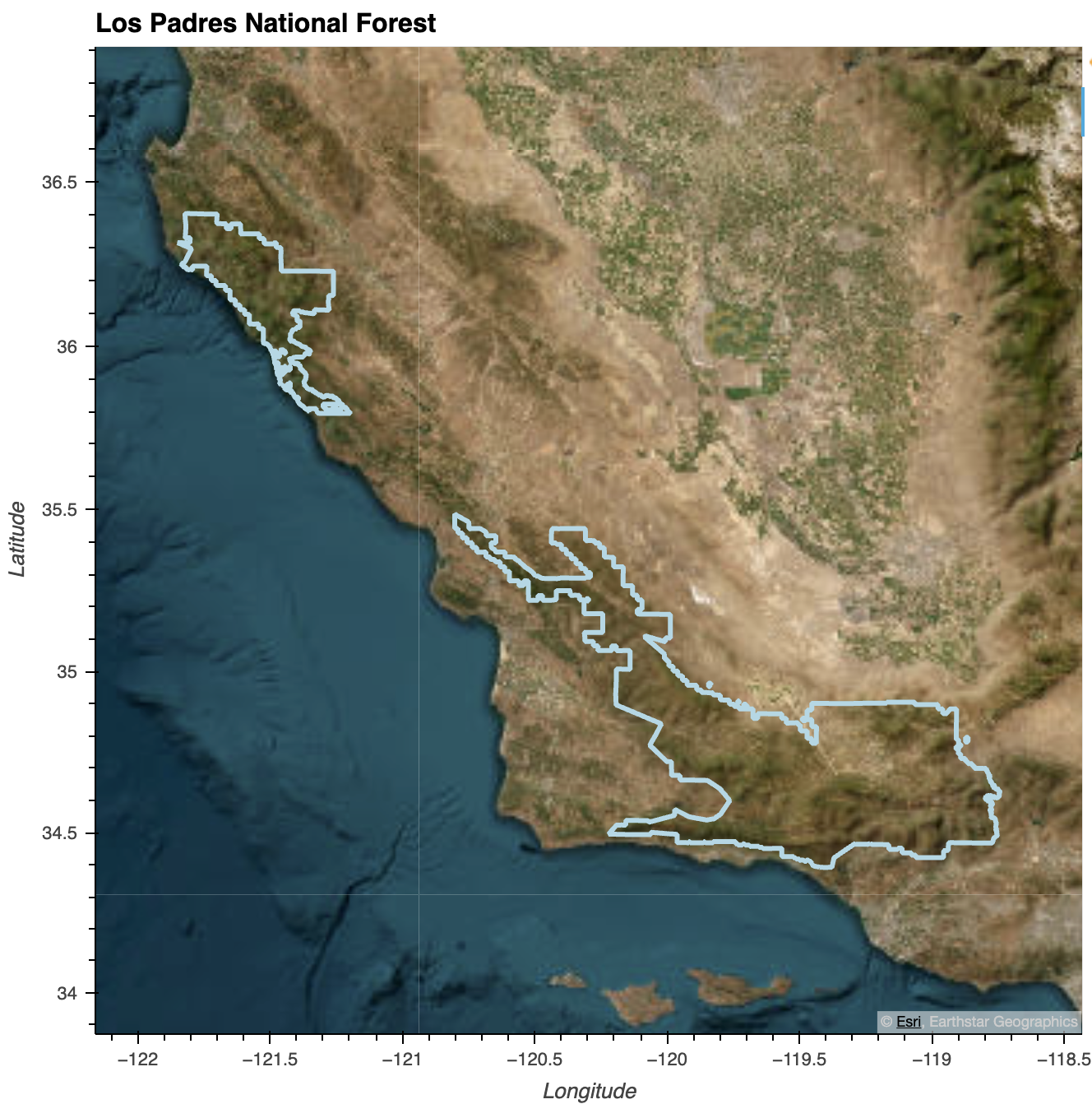
# Los Padres National Forest

los_padres_gdf = all_ca_units.loc[
    all_ca_units['NFSLANDU_2'] == 'Los Padres National Forest'
]
# Create folium map instance
los_padres_gdf.explore()
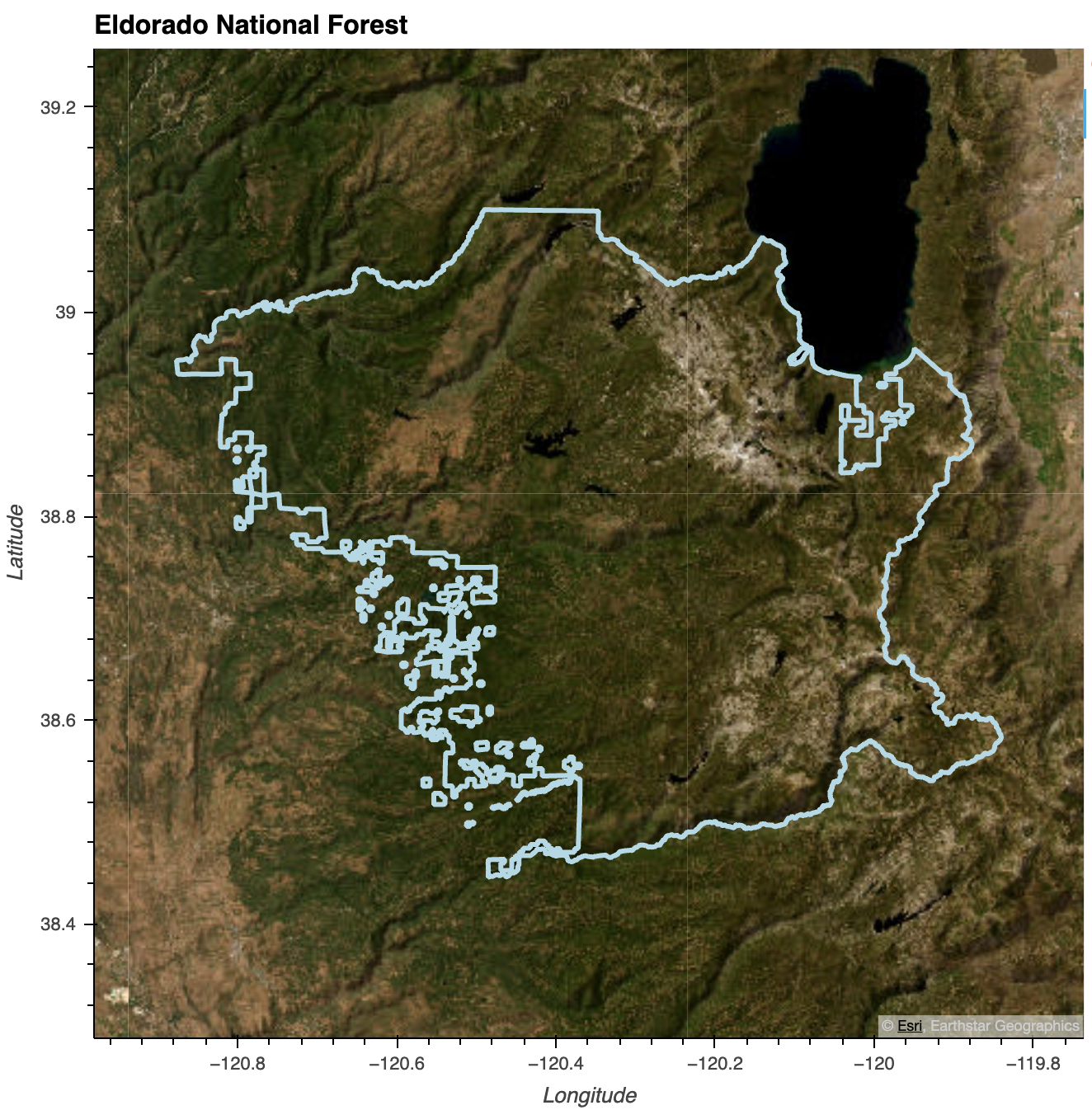
# Eldorado National Forest

eldorado_gdf = all_ca_units.loc[
    all_ca_units['NFSLANDU_2'] == 'Eldorado National Forest'
]

eldorado_gdf.explore()
Retrieve Soils
def create_polaris_urls(soil_prop, stat, soil_depth, gdf_bounds):
    """
    Create POLARIS dataset URLs using site bounds.

    Args:
    soil_prop (str): Soil property.
    stat (str): Summary statistic.
    soil_depth (str): Soil depth (cm).
    gdf_bounds (numpy.ndarray): Array of site boundaries.

    Returns:
    list: A list of POLARIS datset URLs.
    """

    # Get latitude and longitude bounds from site
    min_lon, min_lat, max_lon, max_lat = gdf_bounds

    site_min_lon = floor(min_lon)
    site_min_lat = floor(min_lat)
    site_max_lon = ceil(max_lon)
    site_max_lat = ceil(max_lat)

    all_soil_urls = []

    for lon in range(site_min_lon, site_max_lon):
        for lat in range(site_min_lat, site_max_lat):
            current_max_lon = lon + 1
            current_max_lat = lat + 1

            soil_template = (
                "http://hydrology.cee.duke.edu/POLARIS/PROPERTIES/v1.0/"
                "{soil_prop}/"
                "{stat}/"
                "{soil_depth}/"
                "lat{min_lat}{max_lat}_lon{min_lon}{max_lon}.tif"
            )

            soil_url = soil_template.format(
                soil_prop=soil_prop, stat=stat, soil_depth=soil_depth,
                min_lat=lat, max_lat=current_max_lat,
                min_lon=lon, max_lon=current_max_lon
            )

            all_soil_urls.append(soil_url)

    return all_soil_urls
def download_polaris(site_name, site_gdf, soil_prop, stat, soil_depth,
plot_path, plot_title, data_dir, plots_dir):
"""
Retrieve POLARIS site data, build DataArray, plot site, and export raster.
Args:
site_name (str): Name of site.
site_gdf (geopandas.GeoDataFrame): Site GeoDataFrame.
soil_prop (str): Soil property.
stat (str): Summary statistic.
soil_depth (str): Soil depth (cm).
plot_path (str): Path of topographic plot.
plot_title (str): Title of topographic plot.
data_dir (str): Path of data directory.
plots_dir (str): Path of plots directory.
Returns:
xarray.DataArray: A soil DataArray for a given location.
"""
# Collect site urls
site_polaris_urls = create_polaris_urls(
soil_prop, stat, soil_depth,
site_gdf.total_bounds
)
# Gather site data into a single DataArray
site_soil_da = build_da(site_polaris_urls, tuple(site_gdf.total_bounds))
# Export soil data to raster
export_raster(site_soil_da, f"{site_name}_soil_{soil_prop}.tif", data_dir)
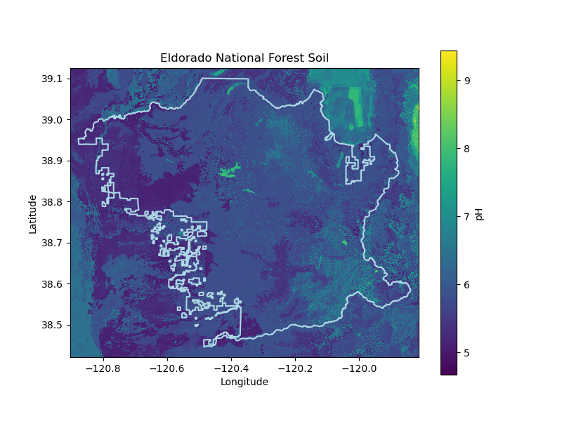
# Create site plot
plot_site(
site_soil_da, site_gdf, plots_dir,
f'{plot_path}-Soil', f'{plot_title} Soil',
'pH', 'viridis', 'lightblue'
)
return site_soil_da
# Set site parameters

soil_prop = 'ph'
soil_prop_stat = 'mean'
# cm (the minimum depth for blue oaks is 1-2 ft)
soil_depth = '30_60'
eldorado_soil_da = download_polaris('eldorado', eldorado_gdf, soil_prop,
                                    soil_prop_stat, soil_depth,
                                    'Eldorado-National-Forest',
                                    'Eldorado National Forest',
                                    data_dir, plots_dir)
los_padres_soil_da = download_polaris('los_padres', los_padres_gdf, soil_prop,
                                      soil_prop_stat, soil_depth,
                                      'Los-Padres-National-Forest',
                                      'Los Padres National Forest',
                                      data_dir, plots_dir)
Select Digital Elevation Model and Calculate Aspect
def select_dem(bounds, site_gdf, download_dir):
    """
    Create elevation DataArray from NASA Shuttle Radar Topography Mission data.

    Args:
    bounds (tuple): Input site boundaries.
    site_gdf (geopandas.GeoDataFrame): Land unit GeoDataFrame.
    download_dir (str): Path of download directory.

    Returns:
    xarray.DataArray: A site elevation raster.
    """

    # Returns data granules for given bounds
    strm_granules = earthaccess.search_data(
        # SRTMGL1: NASA Shuttle Radar Topography Mission
        # Global 1 arc second V003
        short_name="SRTMGL1",
        bounding_box=bounds
    )

    # Download data granules
    earthaccess.download(strm_granules, download_dir)

    # Set SRTM data dir. hgt = height
    strm_pattern = os.path.join(download_dir, '*.hgt.zip')

    # Build merged elevation DataArray
    strm_da = build_da(glob(strm_pattern), tuple(site_gdf.total_bounds))

    return strm_da
def download_topography(site_name, site_gdf, plot_path, plot_title,
                        elevation_dir, data_dir, plots_dir):
    """
    Retrieve topographic data, build DataArray, plot site, and export raster.

    Args:
    site_name (str): Name of site.
    site_gdf (geopandas.GeoDataFrame): Site GeoDataFrame.
    plot_path (str): Path of topographic plot.
    plot_title (str): Title of topographic plot.
    elevation_dir (str): Path of site elevation directory.
    data_dir (str): Path of data directory.
    plots_dir (str): Path of plots directory.

    Returns:
    xarray.DataArray: An elevation DataArray for a given location.
    """

    # Produce Digital Elevation Model DataArray

    elev_da = select_dem(tuple(site_gdf.total_bounds), site_gdf,
                        elevation_dir)
    export_raster(elev_da, f"{site_name}_elevation.tif", data_dir)
    plot_site(
        elev_da, site_gdf, plots_dir, f'{plot_path}-Elevation',
        f'{plot_title} Elevation', 'Meters', 'terrain', 'black',
    )

    # Calculate aspect from elevation

    aspect_da = calculate_aspect(elev_da)
    export_raster(aspect_da, f"{site_name}_aspect.tif", data_dir)
    plot_site(
        aspect_da, site_gdf, plots_dir, f'{plot_path}-Aspect',
        f'{plot_title} Aspect', 'Degrees', 'terrain', 'black'
    )

    return elev_da
eldorado_elev_da = download_topography(
                        'eldorado', eldorado_gdf,
                        'Eldorado-National-Forest',
                        'Eldorado National Forest',
                        eldorado_elevation_dir, data_dir, plots_dir
                    )
los_padres_elev_da = download_topography(
                        'los_padres', los_padres_gdf,
                        'Los-Padres-National-Forest',
                        'Los Padres National Forest',
                        los_padres_elevation_dir, data_dir, plots_dir
                    )
Projected Climate
def get_projected_climate(site_name, site_gdf,
                          emissions_scenario, gcm, time_slices):
    """
    Create DataFrame of projected site climate for a given time period.

    Args:
    site_name (str): Site name.
    site_gdf (dict): Site GeoDataFrame.
    emissions_scenario (str): Climate scenario.
    gcm (str): Global Climate Model.
    time_slices (list): List of years indicating a time slice.

    Returns:
    pandas.DataFrame: A DataFrame of projected average max temperatures.
    """

    maca_das = []

    for start_year in time_slices:
        end_year = start_year + 4

        # Multivariate Adaptive Constructed Analogs (MACA)
        MACA_URL = (
            'http://thredds.northwestknowledge.net:8080/thredds/fileServer/'
            f'MACAV2/{gcm}/macav2metdata_tasmax_{gcm}_r1i1p1_'
            f'{emissions_scenario}_{start_year}_{end_year}_CONUS_monthly.nc'
        )

        maca_da = xr.open_dataset(MACA_URL, engine='h5netcdf').squeeze()

        bounds = site_gdf.to_crs(maca_da.rio.crs).total_bounds

        # update coordinate range
        maca_da = maca_da.assign_coords(
            lon=("lon", [convert_longitude(l) for l in maca_da.lon.values])
        )

        maca_da = maca_da.rio.set_spatial_dims(x_dim='lon', y_dim='lat')
        maca_da = maca_da.rio.clip_box(*bounds)

        maca_das.append(dict(
                            site_name=site_name,
                            gcm=gcm,
                            start_year=start_year,
                            end_year=end_year,
                            da=maca_da))

    return pd.DataFrame(maca_das)
def download_climate(site_name, site_gdf, emissions_scenario,
                     climate_models, time_slices, raster_path, data_dir):
    """
    Retrieve projected site climate for a given time period,
    build composite DataArray, and export raster.

    Args:
    site_name (str): Site name.
    site_gdf (dict): Site GeoDataFrame.
    emissions_scenario (str): Climate scenario.
    climate_models (list): Climate model names.
    time_slices (list): List of years indicating a time slice.
    raster_path (str): Path of site climate raster.
    data_dir (str): Path of data directory.

    Returns: None
    """

    for gcm in climate_models:
        print(f'Downloading climate data for {gcm}')

        # Retrieve MACA climate data
        site_proj_temp = get_projected_climate(
                                        site_name, site_gdf,
                                        emissions_scenario, gcm,
                                        time_slices
                                    )

        # Convert temperature to fahrenheit
        projected_climates_df = site_proj_temp.assign(
                                    fahrenheit=lambda x: x.da.map(
                                        convert_temperature))

        # Create composite site projected climate
        site_clim_composite_ds = xr.concat(
            projected_climates_df.fahrenheit, dim='time').mean('time')

        site_clim_composite_da = site_clim_composite_ds.to_dataarray(
                                    dim='air_temperature',
                                    name='air_temperature')

        export_raster(site_clim_composite_da,
                    f"{raster_path}_{gcm}_max_temp.tif", data_dir)
# Set climate parameters

emissions_scenario = 'rcp45'
climate_models = ['CanESM2', 'MIROC-ESM-CHEM', 'CNRM-CM5', 'GFDL-ESM2M']
mid_century = [2036, 2041, 2046, 2051, 2056, 2061] # 2036-2066
late_century = [2066, 2071, 2076, 2081, 2086, 2091] # 2066-2096
time_periods = [mid_century, late_century]
Eldorado Projected Climate (RCP 4.5)
# Mid century

download_climate('eldorado', eldorado_gdf,
                emissions_scenario, climate_models, mid_century,
                'eldorado_mid_century', data_dir)

# Late century

download_climate('eldorado', eldorado_gdf,
                emissions_scenario, climate_models, late_century,
                'eldorado_late_century', data_dir)
Los Padres Projected Climate (RCP 4.5)
# Mid century

download_climate('los padres', los_padres_gdf,
                emissions_scenario, climate_models, mid_century,
                'los_padres_mid_century', data_dir)

# Late century

download_climate('los padres', los_padres_gdf,
                emissions_scenario, climate_models, late_century,
                'los_padres_late_century', data_dir)
Identify Suitability
def build_habitat_suitability_model(site_name, time_period, gcm,
                                    optimal_values, tolerance_ranges,
                                    data_dir, raster_name):
    """
    Build a habitat suitability model by combining fuzzy suitability scores
    for each variable.

    Args:
    site_name (str): Name of site.
    time_period (str): Name of time period.
    gcm (str): Global Climate Model.
    optimal_values (list): List of optimal values for variables.
    tolerance_ranges (list): List of tolerance values for variables.
    data_dir (str): Path of data directory.
    raster_name (str): The name of model raster.

    Returns:
    str: The path of the suitability raster.
    """
    reference_raster = f"{data_dir}/{site_name}_elevation.tif"

    input_rasters = [
        f"{data_dir}/{site_name}_{time_period}_{gcm}_max_temp.tif",
        f"{data_dir}/{site_name}_aspect.tif",
        f"{data_dir}/{site_name}_soil_ph.tif"
    ]

    harmonized_rasters = harmonize_raster_layers(reference_raster,
                                                 input_rasters, data_dir)

    # Load and calculate suitability scores for each raster
    suitability_layers = []
    suit_zip = zip(harmonized_rasters, optimal_values, tolerance_ranges)
    for raster_path, optimal_value, tolerance_range in suit_zip:
        raster = rxr.open_rasterio(raster_path, masked=True).squeeze()
        suitability_layer = calculate_suitability_score(
                                raster, optimal_value, tolerance_range
                            )
        suitability_layers.append(suitability_layer)

    # Combine suitability scores by multiplying across all layers
    combined_suitability = suitability_layers[0]
    for layer in suitability_layers[1:]:
        combined_suitability *= layer

    # Save the combined suitability raster
    output_file = os.path.join(data_dir, f"{raster_name}.tif")
    combined_suitability.rio.to_raster(output_file)
    print(f"Combined suitability raster saved to: {raster_name}.tif")

    # Path to the final combined suitability raster
    return output_file
# Optimal values for species for each variable
# Variables: elevation, temperature, aspect, soil pH
optimal_values = [1500.0, 90.0, 0.0, 6.75]

# Tolerance ranges (acceptable deviation) for each variable
tolerance_ranges = [1500.0, 20.0, 65.0, 0.75]
Eldorado National Forest Suitability
# CanESM2 (Warm and wet)
build_habitat_suitability_model('eldorado', 'mid_century', 'CanESM2',
optimal_values, tolerance_ranges, data_dir,
'eld_mc_CanESM2_suitability')
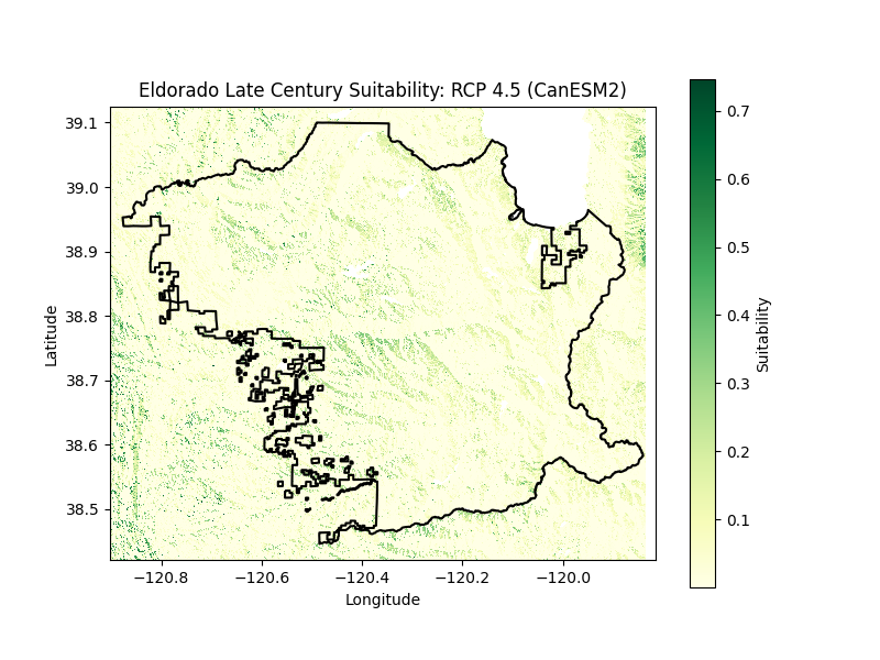
build_habitat_suitability_model('eldorado', 'late_century', 'CanESM2',
optimal_values, tolerance_ranges, data_dir,
'eld_lc_CanESM2_suitability')
# MIROC-ESM-CHEM (Warm and dry)
build_habitat_suitability_model('eldorado', 'mid_century', 'MIROC-ESM-CHEM',
optimal_values, tolerance_ranges, data_dir,
'eld_mc_MIROC-ESM-CHEM_suitability')
build_habitat_suitability_model('eldorado', 'late_century', 'MIROC-ESM-CHEM',
optimal_values, tolerance_ranges, data_dir,
'eld_lc_MIROC-ESM-CHEM_suitability')
# CNRM-CM5 (Cool and wet)
build_habitat_suitability_model('eldorado', 'mid_century', 'CNRM-CM5',
optimal_values, tolerance_ranges, data_dir,
'eld_mc_CNRM-CM5_suitability')
build_habitat_suitability_model('eldorado', 'late_century', 'CNRM-CM5',
optimal_values, tolerance_ranges, data_dir,
'eld_lc_CNRM-CM5_suitability')
# GFDL-ESM2M (Cool and dry)
build_habitat_suitability_model('eldorado', 'mid_century', 'GFDL-ESM2M',
optimal_values, tolerance_ranges, data_dir,
'eld_mc_GFDL-ESM2M_suitability')
build_habitat_suitability_model('eldorado', 'late_century', 'GFDL-ESM2M',
optimal_values, tolerance_ranges, data_dir,
'eld_lc_GFDL-ESM2M_suitability')
Los Padres National Forest Suitability
# CanESM2 (Warm and wet)
build_habitat_suitability_model('los_padres', 'mid_century', 'CanESM2',
optimal_values, tolerance_ranges, data_dir,
'lp_mc_CanESM2_suitability')
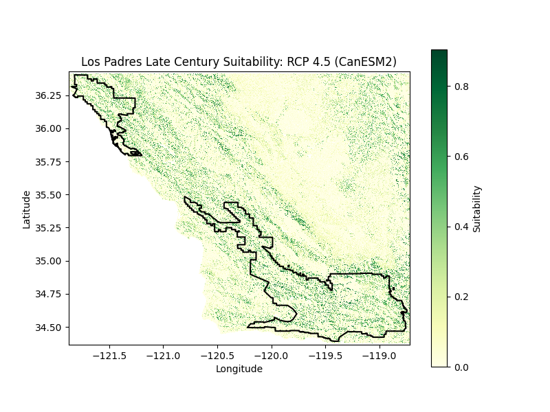
build_habitat_suitability_model('los_padres', 'late_century', 'CanESM2',
optimal_values, tolerance_ranges, data_dir,
'lp_lc_CanESM2_suitability')
# MIROC-ESM-CHEM (Warm and dry)
build_habitat_suitability_model('los_padres', 'mid_century', 'MIROC-ESM-CHEM',
optimal_values, tolerance_ranges, data_dir,
'lp_mc_MIROC-ESM-CHEM_suitability')
build_habitat_suitability_model('los_padres', 'late_century', 'MIROC-ESM-CHEM',
optimal_values, tolerance_ranges, data_dir,
'lp_lc_MIROC-ESM-CHEM_suitability')
# CNRM-CM5 (Cool and wet)
build_habitat_suitability_model('los_padres', 'mid_century', 'CNRM-CM5',
optimal_values, tolerance_ranges, data_dir,
'lp_mc_CNRM-CM5_suitability')
build_habitat_suitability_model('los_padres', 'late_century', 'CNRM-CM5',
optimal_values, tolerance_ranges, data_dir,
'lp_lc_CNRM-CM5_suitability')
# GFDL-ESM2M (Cool and dry)
build_habitat_suitability_model('los_padres', 'mid_century', 'GFDL-ESM2M',
optimal_values, tolerance_ranges, data_dir,
'lp_mc_GFDL-ESM2M_suitability')
build_habitat_suitability_model('los_padres', 'late_century', 'GFDL-ESM2M',
optimal_values, tolerance_ranges, data_dir,
'lp_lc_GFDL-ESM2M_suitability')
Discussion
Habitat suitability for mid and late 21st century was assessed for a medium emissions scenario (RCP 4.5) using four diverging climate models: CanESM2 (Warm/Wet), MIROC-ESM-CHEM (Warm/Dry), CNRM-CM5 (Cool/Wet), and GFDL-ESM2M (Cool/Dry). Species tolerance and optimal ranges for elevation (1,500 ± 1,500 meters), temperature (90 ± 20 °F), aspect (0 ± 65 degrees), and soil (6.75 ± 0.75 pH) were evaluated in site suitability scores. Given the oak’s accommodating tolerance for maximum temperature fluctuations, model differences were minimal between plots and time periods. However, this flexibility does not indicate a robustness to extreme seasonal changes. Blue oaks are generally equipped to withstand drier conditions compared to other native trees, abundant in areas with less conducive soils where they often cohabitate with pines. Nonetheless, the onset of a severe drought diminishes the threshold of site tolerance.
By the end of the century, the average annual maximum temperatures are projected to grow by 7.5°F to 10.9°F. Intense precipitation events are projected as well, with frequencies of pronounced dry seasons and whiplash events expanding by over 50% across the state with a notable change in Southern California: a ~200% increase in extreme dry seasons, a ~150% increase in extreme wet seasons, and a ~75% increase in year-to-year whiplash. Historically blue oak mortality has been typically attributed to decay fungi such as canker rots and root-rotting decay fungi. Pathogens like Phytophthora ramorum, the cause for sudden oak death, respond faster than trees to drought followed by high precipitation events, accelerating disintegration. The combination of disease and long-term climate stress contributes to raised levels of mortality years after drought. Futhermore, although blue oaks have evolved in an environment where fires occur regularly and can survive low-to-moderate intensity fires, the threat of conifer encroachment subjects oaks to more canopy fire risk in a warmer climate.
Sites
Los Padres National Forest is vulnerable to floods and debris flows after extreme precipitation events, in particular after recurrent wildfires, due to the forest’s position in the Coast and Transverse mountain ranges in relation to the coast. Sediment flow in Southern California has a history of high variability under El Niño Southern Oscillation (ENSO) events and has led to the destruction of oak riparian habitat. Eldorado National Forest is similarly projected to experience extreme climate variability between wet and dry years. Toward the end of the century at the lowest and highest elevations in the Sierra Nevada, warming temperatures will lead to greater evaporation and a projected ~15% reduction in fuel and soil moisture. This scenario indicates greater drought likelihood and impacts across native plant communities. Heightened fire weather conditions will generate shifts in blue oak mortality rates as well as post-fire germination. Moreover a shift in oak mortality affects fire activity. Blue oak sites with south-facing aspects in particular demonstrate lower potential for accumulated drainage and thus the highest level of mortality compared to other aspects. Sites like these are especially at risk for greater dead woody surface fuels, enhancing the probability of larger fires over longer periods.
References
Barrett, A., Battisto, C., J. Bourbeau, J., Fisher, M., Kaufman, D., Kennedy, J., … Steiker, A. (2024). earthaccess (Version 0.12.0) [Computer software]. Zenodo. https://doi.org/10.5281/zenodo.8365009
California Native Plant Society (CNPS). (n.d.). Blue oak. https://calscape.org/Quercus-douglasii-(Blue-Oak)
Collins, B., Hetzel, J. T., & Metzger, T. C. (2024). xarray-spatial (Version 0.4.0) [Computer software]. GitHub. https://github.com/makepath/xarray-spatial/releases/tag/v0.4.0
Estes, B. & Gross, S. (2020). Eldorado National Forest climate change trend summary. USDA Forest Service. https://www.fs.usda.gov/Internet/FSE_DOCUMENTS/fseprd985002.pdf
Huesca, M., Ustin, S. L., Shapiro, K. D., Boynton, R., & Thorne, J. H. (2021, June 16). Detection of drought-induced blue oak mortality in the Sierra Nevada Mountains, California. Ecosphere, 12(6). https://doi.org/10.1002/ecs2.3558
Hunter, J. D. (2024). Matplotlib: A 2D graphics environment (Version 3.9.2) [Computer software]. Zenodo. https://zenodo.org/records/13308876
Jordahl, K., Van den Bossche, J., Fleischmann, M., Wasserman, J., McBride, J., Gerard, J., … Leblanc, F. (2024). geopandas/geopandas: v1.0.1 (Version 1.0.1) [Computer software]. Zenodo. https://doi.org/10.5281/zenodo.12625316
Molinari, N., Sawyer, S., & Safford, H. (n.d.). A summary of current trends and probable future trends in climate and climate-driven processes in the Los Padres National Forest and neighboring lands. USDA Forest Service. https://www.fs.usda.gov/Internet/FSE_DOCUMENTS/fseprd497638.pdf
Point Blue Conservation Science. (n.d.). California oak planting guide. https://www.pointblue.org/wp-content/uploads/2023/06/Planting-Oaks-Guide-Version-1.pdf
Python Software Foundation. (2024). Python (Version 3.12.6) [Computer software]. https://docs.python.org/release/3.12.6
Rudiger, P., Liquet, M., Signell, J., Hansen, S. H., Bednar, J. A., Madsen, M. S., … Hilton, T. W. (2024). holoviz/hvplot: Version 0.11.0 (Version 0.11.0) [Computer software]. Zenodo. https://doi.org/10.5281/zenodo.13851295
Sacramento Valley Chapter (CNPS). (n.d.). Oak woodland. https://www.sacvalleycnps.org/oak-woodland/#:~:text=Habitat%20Values,and%20streams%20for%20anadromous%20fishes
Snow, A. D., Scott, R., Raspaud, M., Brochart, D., Kouzoubov, K., Henderson, S., … Weidenholzer, L. (2024). corteva/rioxarray: 0.18.1 Release (Version 0.18.1) [Computer software]. Zenodo. https://doi.org/10.5281/zenodo.4570456
Swain, D. L., Langenbrunner, B., Neelin, J. D., & Hall, A. (2018). Increasing precipitation volatility in twenty-first-century California. Nature Climate Change, 8(5), 427. https://doi.org/10.1038/s41558-018-0140-y
Swiecki, T. & Bernhardt, E. (2020). Recent increases in blue oak mortality. Phytosphere Research. https://oaks.cnr.berkeley.edu/wp-content/uploads/2020/04/Swiecki-Bernhardt-Oak-Mortality-4.2-2020.pdf
Tallamy, D. W. (2021). The nature of oaks: The rich ecology of our most essential native trees. Timber Press.
The pandas development team. (2024). pandas-dev/pandas: Pandas (Version 2.2.2) [Computer software]. Zenodo. https://doi.org/10.5281/zenodo.3509134
UC Oaks. (n.d.). Blue oak-foothill pine woodland & wildlife habitat. https://oaks.cnr.berkeley.edu/blue-oak-foothill-pine-woodland-wildlife-habitat
UC Oaks. (n.d.). Coastal oak woodland & wildlife habitat. https://oaks.cnr.berkeley.edu/coastal-oak-woodland/
UC Oaks. (n.d.). Conifer encroachment. https://oaks.cnr.berkeley.edu/conifer-encroachment/
UC Oaks. (2024, July 1). Oak tree species ID & ecology. https://oaks.cnr.berkeley.edu/oak-tree-species-id-ecology
University of California Merced (n.d.). Future Climate Scenarios. The Climate Toolbox. https://climatetoolbox.org/tool/Future-Climate-Scenarios
USDA Forest Service. (n.d.). About the area. https://www.fs.usda.gov/main/eldorado/about-forest/about-area
USDA Forest Service. (n.d.). About the forest. https://www.fs.usda.gov/main/lpnf/about-forest
USDA Forest Service. (n.d.). Quercus douglasii. https://www.fs.usda.gov/database/feis/plants/tree/quedou/all.html
USDA Southern Research Station. (n.d.). Quercus douglasii. https://www.srs.fs.usda.gov/pubs/misc/ag_654/volume_2/quercus/douglasii.htm